Module Components

• Overview

Topics

• T-TESTS
• Mann-Whitney U and Wilcoxon Signed-Ranks Tests

NRSG 795: BIOSTATISTICS FOR EVIDENCE-BASED PRACTICE

Module 5: Significance Testing/Hypothesis Testing for Two Groups

T-TESTS

A common statistical test is testing if the means of two groups are statistically different. A t-test asks whether a difference between two groups’ averages is unlikely to have occurred because of random chance in sample selection (click for visuals). The null hypothesis is Ho: μ1 = μ2, and the hypothesis being tested is μ1 ≠ μ2.x

This test involves two variables: 1) one of the variables usually the independent variable describes our groups. The grouping variable can only have two groups (dichotomous) and must be mutually exclusive. 2) the other variable is the characteristic (outcome/dependent variable) that we are interested in exploring whether a difference exists. This variable must be normally distributed and continuous.  An example of a research question could be – are there gender (grouping variable: male or female) differences in how many calories one eats per day? The grouping variable in an intervention/experimental trial would be the intervention/experimental group vs the control/ treatment as usual group. The grouping variable can also capture a ‘time’ component such as pretest or posttest. 

A difference is more likely to be meaningful and "real" if

1. the difference between the averages is large,
2. the sample size is large, and
3. responses are consistently close to the average values and not widely spread out (the standard deviation is low).

t-value

The t test quantifies the difference between two means based on the amount of variance in both groups. Using the calculated t-value (test statistic), degrees of freedom and an alpha=0.05 one can look up the critical value that corresponds to the calculated t value to obtain a p-value (e.g., Munro book Appendix C) or most statistical software programs provide the exact p-value for you.

Thinking it through:

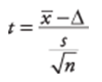
1. When you perform a t-test you will obtain a computed t-value (also referred to as t-stat) This t-value is derived using the formula above and your data.
2. You should have already determined if using an one or two tail test and level of significance (in most cases one uses a two tailed test with the level of significance of 0.5)
3. Then the computed t-value is compared to a critical value
1. If the absolute value of the computed t-value is < than the t critical value the p-value is going to be >.05 meaning the groups are not different
2. If the absolute value of the computed t-value is > than the t critical value the p-value is going to be <.05 meaning group differences exist

Types of t-test (examples)

• Independent groups: When there are two independent groups, an independent t-test is done.
• Dependent groups: When the means for one group at two different times are compared, a paired or dependent t-test is done. The groups can be the same individuals measured before and after an intervention (pre/post), or when one group is ‘paired’ with another, such as twins, husbands and wives, fathers and sons.
• Click here if you want to see ‘behind the scenes’ of what is going on via hand calculating t tests

Test Assumptions

There are certain assumptions that must be met for the results of a t-test to be valid. These assumptions are:

1. Participants have been randomly sampled (this is often violated).
2. Variables have the correct level of measurement. The dependent variable is measured at the interval or ratio level and the independent variable is nominal (group).
3. The dependent variable is normally distributed.
• One way to get a rough estimate of this is to evaluate whether the measures of central tendency are approximately equal.
• A more formal way is to use the Shapiro-Wilk test (click for more information on other ways to detect normality in distributions) that is provided by some software programs like IntellectusStatistics. The test gives you a W value; small values of W indicate your sample is >notnormally distributed. Thus you reject the null hypothesis that your population is normally distributed if your values are under a certain threshold.
  
  Note for this course the central tendency measure evaluation can be used by everyone, regardless of which software you have chosen.
4. The variances in the groups being compared are similar. This is called homogeneity of variance or homoscedasticity.
   • One way to get a rough estimate of whether population variances are equal is to compare the standard deviations between the two groups. If the variances are similar, then the standard deviations (i.e., square root of variance) should be similar.
   • There are two formulas to calculate independent t –tests and which one to use is determined on whether the variances of the groups being compared are equal (independent t test for pooled samples) or if the variances differ (independent t test for separate samples).
   • A more formal way is to use the Levene’s test (click for more information) that is provided by some software programs like IntellectusStatistics. If the resulting p-value of Levene's test is less than some significance level (typically 0.05), the obtained differences in sample variances are unlikely to have occurred based on random sampling from a population with equal variances. Thus, the null hypothesis of equal variances is rejected and it is concluded that there is a difference between the variances in the population. When Levene's test shows significance, one should switch to generalized tests (non-parametric tests), free from homoscedasticity assumptions. Note that we will not use Excel to conduct the Levene’s test in this class and it is not expected on the assignments or exam.

If one or more of the assumption of a t test are not met the conclusions may be threatened because the computed p-value may not be correct.  However, one can still use the t test with confidence when assumptions are only somewhat violated in such cases as when the sample size is large (>30 cases), the data are not badly skewed, and there is a fairly large range of values across the continuous variable.

Effect size

The magnitude of a relationship in analyses using independent group t test is communicated in the form of Cohen’s d (also called the standardized mean difference). Cohen’s d is easy to compute:

Cohen (1988) has provided guidelines to describe the absolute value of the effect size: 0.2 small, 0.5 medium, 0.8 large.

Presenting results

This is an example of how results may be written for an independent samples t-test: An independent samples t-test was conducted to compare self-esteem scores for males and female high school students. There was no significant difference in mean scores for males (M=34.1, SD=4.9) and females (M=33.2, SD=5.7); t=1.62, p=.11, two tailed.

This is an example of how results may be written for a paired samples t-test : A paired samples t-test was conducted to evaluate the impact of the weight loss intervention on women’s confidence in ability to lose weight. There was a statistically significant increase in confidence from baseline (M=55.2, SD=5.8) to three months after the intervention (M=68.5, SD= 5.0); t=5.39, P<.0005, one-tailed.

Note: Is is important when you summarize the statistical data that you include the means and standard deviations of the groups being compared, as well as the test statistic, and p-value. By providing the means even someone with no statistical background can get an idea of the results of whether the means are similar to one another or if different and which direction.

Required Videos

• Independent samples t-test:   https://www.youtube.com/watch?v=jyoO4i8yUag  (6:52)
• Dependent Samples t- test:  https://www.youtube.com/watch?v=zD3VIBkwc-0 (4:58)

• NOT REQUIRED: article with more information

Learning Activities

• Determine which t-test you would perform to test these research questions and check your answers here.
• Practice interpreting findings by answering these questions using the table below.
  
  
  
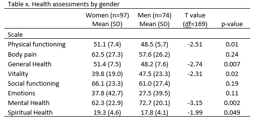
  Check your answers here.
• Practice how to run an independent t-test. The Excel file HeartFailure_n=30.xlsx contains data from a study of 30 patients hospitalized with heart failure who participated in a randomized trial of three treatments: enhanced teaching in hospital, usual care in hospital, and enhanced teaching with home care. You will answer the question: Is there a significant difference between males and females in the Heart Failure Self-care Index scores? What is your evidence (e.g., t-statistic, p-value)?
  (note about the datafile: Click on the “Labels” tab in the workbook to see the variable names and value labels (aka coding). The “data” tab shows how data are often displayed with one row representing each person. )

• Check your answers to the steps in testing the heart failure hypothesis.

Guide for those choosing to use IntellectusStatistics	Guide for those choosing to use Excel
Refer to the hint sheet and videos for how to run a t-test Hints to running t tests in IS Independant T-test Paired samples t-test	Two Means t-tests in Excel (3:53) Hints to running t tests in EXCEL The “t-test” tab shows the results of sorting the data and creating columns for females and males so that a t-test can be calculated. Delete the t-test results and run your own analyses comparing the Heart Failure Self-care Index scores for males and females following the instructions in the Excel video.