Module Components

• Overview

Topics

• Partial Correlation
• Modeling Independent Variables in Regression Models
• Multiple Linear Regression
• Multiple Logistic Regression

NRSG 795: BIOSTATISTICS FOR EVIDENCE-BASED PRACTICE

Module 9: Model Building-Multiple Independent Variables

Modeling Independent Variables in Regression Models

Previously we focused on simple linear and logistic models. This meant the models were testing the relationship between only one independent variable and our outcome. We tended to also use continuous type independent variables (interval/ratio) in our examples because it enabled you to see the connection to similar principles that applied to correlation. In this module, we expand on what we learned about simple regression models by learning more about data handling issues and strategies used when including multiple independent variables (also referred to as covariates) in regression models.

Variable types and data coding (Dummy variables)

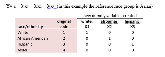
Continuous independent variables can be entered into models as they are and as we saw previously the beta coefficient is interpreted based on the sign and magnitude. For example: “for each point increase in locus of control perceived stress decreased by 2.4 points (beta= -2.4, p=.01).” Interval/ratio level of measurement can also be reconfigured or coded as nominal/ordinal level variables. When using nominal/ordinal variables one needs to know what the ‘reference’ group is. In other words what is the group everyone else will be compared to. For example, a dichotomous variable like gender has two groups. One group, say male, is coded as a value of ‘0’ while females are coded as ‘1’. When we insert this variable into a regression model the output expresses the coefficient value for females as compared to the reference group males.

Thus, nominal level variables must be coded in a manner that allows appropriate interpretation of the coefficient. A widely used scheme for recoding is called dummy coding. Dummy coding is specifically important for nominal level measurements with more than one category. The idea behind it is that one creates a series of dichotomous variables that contrast members in one category with everyone else who are the reference (see below matrix). The dummy variables act like 'switches' that turn various parameters on and off in an equation. We create c-1 new variables, where c represents the number of original categories.

The following two videos show how dummy variables are created from a single variable representing treatment.  The second explains how dummy variables are entered into a linear regression model and how they are interpreted.

• How to create a set of dummy variables for regression (6:12)
  http://www.youtube.com/watch?v=Nc-0QdQk01s
• K or K-1 dummy variables for regression (5:40)
  http://www.youtube.com/watch?v=YY9WQG3FsfM

Influential Cases

(visual)

As we learned in correlation one should check the assumption of an absence of influential cases. Typically points further than, say, three or four standard deviations from the mean are considered as “outliers”. An outlier is an extreme observation or a point that differs substantially from the main trend of the data. In regression, these outlying data points can affect the estimated slope and intercept results. When outliers occur, it does not mean these points should be eliminated just to fit your regression as this may end up destroying some of the most important information in your data. Instead it means to look for errors or perhaps a better understanding of what is the cause.
What do you do to avoid having outliers influence you results?

• First review the data. Try to assess whether substantive information exists to help understand the situation, e.g., entry mistake, special circumstance, measurement error.
• An alternative is to perform the regression both with and without the outliers and reflect on the influence on the results.

Multicollinearity

Before throwing data about every potential predictor under the sun into your regression model, we need to think about something known as  multicollinearity. With regression there comes a point where adding more is not better. Independent variables (x’s) are often very correlated with each other and if you put them in the model together the results may be unstable cause they are fighting each other for their unique effect. Multicollinearity occurs when your model includes multiple independent variables that are highly correlated to each other. In other words, it results when you have independent variables that are a bit redundant. Low levels of collinearity pose little threat to regression models, however, highly correlated (>.8) variables can create unstable regression coefficients (overinflates SE).

What do you do to avoid multicollinearity?

• Evaluate the correlation between each of your independent variables (bivariate associations) before including them into the model and if highly correlated only enter one of them into your model.
• Some software programs provide a variance inflation factor (VIF), which assesses how much the variance of an estimated regression coefficient increases if your predictors are correlated.  If no factors are correlated, the VIFs will all be 1, but if the VIF is greater than 1, the predictors may be moderately correlated.

Strategies for entering predictors

In simple regression models one is only entering one independent variable so you don’t need to worry about what order to include it. When dealing with multiple covariate, selecting a method for entering variables into the model is important as it depends on whether you want the order of entry to be based on theoretical rather than statistical rationale (strategies). Type I error is increased when using stepwise solutions.

• Standard approach/simultaneous-enter all at once
• Hierarchical entry-force the order using predetermined sets of variables
• Stepwise (forward or backward)-variables are entered and assessed individually at each step and dropped if contribution is not significant

Model Fit

Fitting a model means obtaining estimators for the unknown population parameters. A well-fitting regression model results in predicted values close to the observed data values.

The statistics used in Ordinary Least Squares (OLS) regression (linear) to evaluate model fit include: R-squared and the overall F-test.

• R-squared has the useful property that its scale is intuitive: it ranges from zero to one, with zero indicating that the proposed model does not improve prediction. In models with more than one predictor variable one should use the Adjusted R-squared. The "adjusted R²" is intended to "control for" overestimates of the population R² resulting from small samples, high collinearity or small subject/variable ratios. When the interest is in the relationship between variables, not in prediction, the R-square is less important.
• The F-test evaluates the null hypothesis that all regression coefficients are equal to zero versus the alternative that at least one does not. An equivalent null hypothesis is that R-squared equals zero. A significant F-test indicates that the observed R-squared is reliable, and is not a spurious result of oddities in the data set. Thus, the F-test determines whether the proposed relationship between the response variable and the set of predictors is statistically reliable, and can be useful when the research objective is either prediction or explanation.

In logistic regression one often uses goodness-of-fit (GOF) tests, such as the Pearson chi-square, or the Hosmer-Lemeshow test, which can help you decide whether your model is correctly specified. GOF tests produce a p-value. If it’s low (say, below .05), you reject the model. If it’s high, then your model passes the test a goodness-of-fit statistic indicating a better fit.

Residual Analysis

Residual analyses can be used to check assumptions and model fit, especially those important to linear regression. A histogram of standardized residuals is often used to examine if the relationships are linear and if the dependent variable is normally distributed. Plotting residuals against the predicted values and independent variables lets one examine the homoscedasticity assumption that for each value of x the variability of the y is about the same and vice versa.

Sample Size and the Number of Covariates

Care should be taken to ensure an adequate sample size for regression models that involve multiple covariates. In practice it is best to achieve a parsimonious model with strong predictive power using a small set of good predictors. A large number of predictors increases the risk of a Type I error and may also result in problems with collinearity.

Steps In Conducting A multivariate Regression Analysis

Building a model that contains several variables is a complex process that requires careful planning. Below are some general procedural steps to follow when building a model:

1. Define the hypothesis being tested
   • Specify the dependent and independent variables
   • Determine the level of measurements
   • Run univariate frequencies and obtain the appropriate descriptive statistics.
   • Check for out of range codes
   • Recode variables as needed (e.g., create dummy coding if necessary)
2. Run the bivariate analysis
   • Test the relationship between each independent variable and the dependent variable
   • Examine the relationships between the independent variables –looking of multicollinearity or variables that are almost identical in cross-tabulations.
3. Run the full model
   • Refer back to hypothesis of what you want to do
   • Correctly specify the dependent variable appropriate for the type of model (linear vs logistic regression)
   • Check assumptions of the model
   • Choose the independent variables based on theory and on the bivariate results
   • Plan to include some sociodemographic variables in the model as these are often important confounding variables.
4. Review the model
   • Assess the statistical significance of the overall model and the individual predictors
   • Discuss the practical significance of the results