Online Course
NRSG 795: BIOSTATISTICS FOR EVIDENCE-BASED PRACTICE
Module 3: Variation and the Normal Distribution
The Normal Distribution
The characteristics of the normal distribution provide the basis for many inferential statistics. The normal distribution is unimodal, symmetric and not too peaked or flat; it is also known as the bell curve and the total area under the curve is equal to 1. In a normal distribution the mean=median=mode. The baseline of the normal curve is measured off in SD units. We often express values as 1 or 2 SD above and below the mean. If you had a mean score of 100 and a SD of 34, 1 SD above the mean would be 100+34 and 1 SD below the mean 100-34 indicating values between 66-134 are within 1 SD of the mean. Remember the mean indicates the best single point in the distribtuion but the SD tells us on average how much the values deviate from the mean. Another way to interpret it would be to say the values between 66-134 are closer to the mean on average while values greater than 1 SD away are further from the mean than the average.
If normality can be assumed, there are known probabilities associated with the distribution. For example, in a normal distribution, 68% of the observations fall between -1 and +1 standard deviations from the mean.
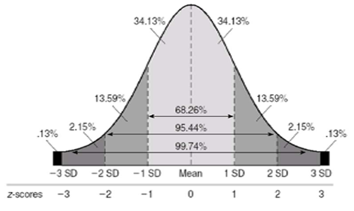 In a Normal curve
95% of the scores will be within 1.96
standard deviations of the mean
[95%] Mean ± 1.96 (2 SD)
99% of the scores are within
2.58 standard deviations
[99%] Mean ± 2.58 (3 SD)
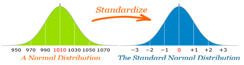
Standardized scores (Z scores)
Likewise, knowing that a particular variable has a normal distribution, if you are given the mean and the standard deviation, you can determine where a particular score lies on the distribution. This is done by calculating a standardized score (z score: Standard scores have a mean of 0 and an SD of 1.0) and comparing it to a table that tells what proportion of the observations lie above (or below) that score. This is like a percentile score that you might have received in taking a standardized exam (click for more information). Z scores are useful when you want to compare things on different metrics (e.g, height and weight). Standard scores have a mean of 0 and an SD of 1.0.
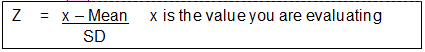
One can then use z scores to compute percentile ranks that describe a given score in relation to other scores in the distribution. After the z score value is computed, we can look up the z-score in a z-table by looking up the first digit and first decimal place in the column labeled ‘z’. Then find the hundredth decimal place across the top row of the table. The number found at the intersection of the row and column identified is the percentage of the area under the curve between the z score and the mean(0). Illustrated at http://www.z-table.com/how-to-use-z-score-table.html.
| How to Calculate Using Excel | Other Resources |
|---|---|
type =standardize (x, Mean, SD) in a cell on the worksheet to calculate the z-score type =normSdist(insert the z-score) in another cell to calculate the percent above or below. |
Online calculator: https://www.zscorecalculator.com/
How to use a Z score table http://www.z-table.com/how-to-use-z-score-table.html |
The Central Limit Theorem which states that if a large number of samples are taken from a population, the means of the samples when plotted will approximate the normal distribution. The videos address the same topics but with a particular focus on z-scores and reading z-tables.
Required Videos
Learning Activity
This website is maintained by the University of Maryland School of Nursing (UMSON) Office of Learning Technologies. The UMSON logo and all other contents of this website are the sole property of UMSON and may not be used for any purpose without prior written consent. Links to other websites do not constitute or imply an endorsement of those sites, their content, or their products and services. Please send comments, corrections, and link improvements to nrsonline@umaryland.edu.