Module Components

• Overview

Topics

• Describe Associations: Cross Tabulation/
  Contingency/Pivot Tables
• Statistically Testing Association: Chi-Square
• Measuring Disease
• Simple Logistic Regression

NRSG 795: BIOSTATISTICS FOR EVIDENCE-BASED PRACTICE

Module 8: Associations Between Nominal or Ordinal Variables

Simple Logistic Regression

What if after viewing your scatterplot you cannot assume a linear relationship? What if your outcome variable is not continuous or does not have a normal distribution yet you still want to quantify the magnitude of an association? Then we can use Simple Logistic Regression when we have one nominal variable (dependent variable) and one independent variable, and you want to know whether variation in the independent variable causes variation in the nominal variable.

Similar to the way linear regression techniques expand our arsenal of tools to investigate continuous outcomes, the logistic regression model generalizes contingency table methods for binary outcomes. The basic structure mirrors that of the linear regression model. The logistic regression model provides an estimate (much like the β in linear regression) that is then exponentiated (e^β)  and we understand as the odds ratio [click here for more information on comparing to linear regression and other information].

A Simple Logistic Regression estimates what is referred to as the unadjusted (or crude) odds ratio—that is the Odds ratio without controlling for other variables. This estimate is exactly the same as the odds ratio calculated from the 2x2 table using the formula ad/bc. 

The equation for a Simple Logistic Regression looks like this: ln[P(Y=1/P(Y=0)] =a+bX

The interpretation of the coefficients for different types of independent variables is as follows (e^β= odds ratio):

• If X is a dichotomous variable with values of 1 or 0, then the b coefficient represents the log odds that an individual will have the event for a person with Xj=1 versus a person with X=0.
• If X is a continuous variable, then the eb represents the odds that an individual will have the event for a person with X=m+1 versus an individual with X=m. In other words, for every one unit increase in X, the odds of having the event Y changes by eb.

In logistic regression the DV is binary (e.g., yes/no) and the DV is transformed into the natural log of the odds (the natural logarithm of the odds for each level of X, designated as "log odds"), which is called a logit (short for logistic probability unit). Probabilities ranging between 0.0 and 1.0 are transformed into odds ratios that range between 0 and infinity.  The mechanics of the process begin with the log odds, which will be equal to 0.0 when the probability in question is equal to .50, smaller than 0.0 when the probability is less than .50, and greater than 0.0 when the probability is greater than .50.

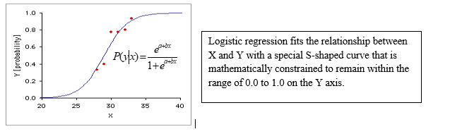
Simple Logistic Regression finds the equation that best predicts the value of the Y variable for each value of the X variable. What makes logistic regression different from linear regression is you do not measure the Y variable directly; instead it is the probability of obtaining a particular value of a nominal variable. You find the slope (b) and intercept (a) of the best-fitting equation in a logistic regression using the maximum-likelihood method, rather than the least-squares method you use for linear regression. Maximum likelihood is a computer-intensive technique; the basic idea is that it finds the values of the parameters under which you would be most likely to get the observed results by using an iterative procedure starting with an initial estimate and then the MLE algorithm determines the direction and size of change in the logit coefficients. The goal is to determine the best combination of predictors to maximize the likelihood of obtaining the observed frequencies on the outcome variable.

Note: You can also analyze data with one nominal and one continuous variable using a one way ANOVA or t-test, and the distinction can be subtle. One clue is that logistic regression allows you to predict the probability of the nominal variable. For example, imagine that you had measured the cholesterol level in the blood of a large number of 55-year-old women, then followed up ten years later to see who had had a heart attack. You could do a t–test, comparing the cholesterol levels of the women who had heart attacks vs. those who didn't, and that would be a perfectly reasonable way to test the null hypothesis that cholesterol level is not associated with heart attacks; if the hypothesis test was all you were interested in. However, if you wanted to predict the probability that a 55-year-old woman with a particular cholesterol level would have a heart attack in the next ten years, so that you could tell your patients "If you reduce your cholesterol by 40 points, you'll reduce your risk of heart attack by X%," you would have to use logistic regression.

Specifications and Assumptions

Logistic regression requires the dependent variable to be binary and coded so that P(Y=1) is the probability of the event occurring, thus it is necessary that the dependent variable is coded accordingly (1=event/yes). Because maximum likelihood estimates are less powerful than ordinary least squares (e.g., simple linear regression) a larger sample size is required. It is recommended that there are at least 30 cases for each parameter to be estimated.

The two main assumptions are:

1. Error terms are assumed to be independent (not appropriate for within-subject or matched-paired designs)
2. the independent variables are linearly related to the log odds

Essentially logistic regression is less restrictive than linear regression. Differences from linear regression as • does not need a linear relationship between the dependent and independent variables

• a linear relationship between the dependent and independent variables is not needed
• no need to meet the normality assumptions (the independent variables do not need to be multivariate normal – or the error terms (the residuals) do not need to be multivariate normally distributed.
• homoscedasticity is not needed

Effect Size

The effect size measures typically used in categorical data analysis are:

1. Odds Ratio (OR)
2. Relative Risk (RR) or Risk Ratio or probability ratio
3. absolute risk reduction (ARR)"

Presenting Results

Example of how results may be written for a Simple Logistic Regression:

Participants who were not offered an incentive at the time of collection (interview) were twice as likely to decline to a blood draw than those who were offered an incentive at the time of collection (96.1 % versus 91.2% respectively, (OR= 2.35, 95% CI= 1.39, 3.99; p=0.001).

Note: Similar to chi square results it is useful if the description can also include a comparison of percentages in addition to the odds ratio estimate and 95% confidence interval. One does not have to present BOTH the 95% confidence interval and the p-value cause confidence intervals trapping 1.0 will not be significant. The 95% confidence interval is preferred over the p- value cause p-values are dependent on sample size.

Required Videos

• Simple Logistic Regression (17:30) https://www.youtube.com/watch?v=_Po-xZJflPM

Additional Information

• Example problem
• Article review about logistic regression

Learning Activity

• Complete the Module 8 self test.